Gaussian Process Latent Variable Models

Posted Jul 7, 2023 Updated Jan 27, 2024

By Alexander Manlove 26 min read

A look at the mathematical underpinnings of the standard Gaussian Process Latent Variable Model, as proposed by Lawrence [2005]. This is an expressive Bayesian latent variable model which employs a nonparametric generative decoder by placing a Gaussian Process prior on the mapping function between latent space and data space.

Gaussian Processes

A Gaussian process (GP) is a distribution over functions and is commonly described as the infinite-dimensional generalisation of a multivariate normal distribution.

Formally, a Gaussian process is a stochastic process defined on a $D$-dimensional input space $\mathcal{X} \subseteq \mathbb R^D$, which assigns to each $\mathbf x \in \mathcal{X}$ a random variable $f(\mathbf x)$, such that for each finite subset $\mathbf X = {\mathbf x_1, \ldots, \mathbf x_N} \subseteq \mathcal{X}$, the distribution over the vector of random variables $f (\mathbf X) = [f(\mathbf x_1), \ldots, f(\mathbf x_N)]^T$ is multivariate Gaussian.

A Gaussian process is fully characterised by its mean function $\mathcal M: \mathcal{X} \rightarrow \mathbb{R}$ and covariance (or kernel) function $\mathcal K: \mathcal{X} \times \mathcal{X} \rightarrow \mathbb{R}$. The mean function provides a measure of central tendency for the process, while the covariance function provides a measure of similarity between the function values at different points in the input space. Typically, we denote a Gaussian process prior using the following notation:

\[f \sim \mathcal{GP}(\mathcal M(\mathbf x), \mathcal K(\mathbf x, \mathbf x'))\]

This expresses that the random variable $f$, is drawn from a Gaussian process with mean function $\mathcal M(\mathbf x)$ and covariance function $\mathcal K(\mathbf x, \mathbf x’)$. By the GP definition above, for a finite set of inputs $\mathbf X = {\mathbf x_1, \mathbf x_2, …, \mathbf x_N}$, the corresponding vector of function values $f(\mathbf X) = [f(\mathbf x_1), f(\mathbf x_2), …, f(\mathbf x_N)]^T$ is normally distributed.

Hence, we can equivalently write: $f(\mathbf X) \sim \mathcal N(\boldsymbol{\mu},\mathbf K),$ where $\mathcal{N}(\cdot,\cdot)$ denotes the multivariate Gaussian distribution. The mean vector $\boldsymbol{\mu}$ is given by evaluating the mean function $\mathcal M(\mathbf x)$ at all $\mathbf x$ in $\mathbf X$, i.e. $\boldsymbol{\mu} = \mathcal M(\mathbf X) = [\mathcal M(\mathbf x_1), \mathcal M(\mathbf x_2), …, \mathcal M(\mathbf x_N)]^T \in \mathbb R^N$. The matrix $\mathbf K = [\mathcal K(\mathbf x_i, \mathbf x_j)]_{i,j=1}^{N} \in \mathbb R^{N\times N}$ is the symmetric positive-semidefinite kernel matrix constructed by evaluating the kernel function $\mathcal K(\mathbf x, \mathbf x’)$ at each pair of points in $\mathbf X$. Often we take the zero function as our prior mean function because it simplifies computations without loss of generality.

Kernel Functions

For a multivariate normal distribution, the covariance matrix quantifies the degree of statistical dependence between dimensions at fixed indices. By contrast, in a GP model, the kernel function provides a measure of similarity between function values for any two given points in the input space. Broadly speaking, these kernel functions quantify the degree to which function values that are near each other in the input space are similar in the output space. Through careful specification of the kernel function, we can incorporate prior beliefs about the properties of the functions we want to learn, such as smoothness or periodicity.

Kernel functions depend on hyperparameters which govern the properties of the function instances drawn from the Gaussian process. These hyperparameters significantly affect the performance of the Gaussian process model and need to be chosen carefully. The table below provides a brief summary of popular kernel functions and their associated hyperparameters.

Name	Kernel Params, $\theta$	Function Equation
Linear	signal variance $s$	$\mathcal K(\mathbf{x}, \mathbf{x}’) = s \mathbf{x}^T \mathbf{x}’$
Squared Exponential	length scale $l$, signal variance $s$	$\mathcal K(\mathbf{x}, \mathbf{x}’) = s \exp \left( -\frac{\lvert{}\lvert{}\mathbf{x} - \mathbf{x}’\rvert\rvert^2}{2l^2} \right)$
Matérn	length scale $l$, signal variance $s$, smoothness $\nu$	$\mathcal K(\mathbf{x}, \mathbf{x}’) = s \left(\frac{2^{1-\nu}}{\Gamma(\nu)}\right) \left( \frac{\sqrt{2\nu} \lvert{}\lvert{}\mathbf{x} - \mathbf{x}’\rvert\rvert}{l} \right)^\nu K_\nu \left( \frac{\sqrt{2\nu} \lvert{}\lvert{}\mathbf{x} - \mathbf{x}’\rvert\rvert}{l} \right)$
Rational Quadratic	length scale $l$, signal variance $s$, shape parameter $\alpha$	$\mathcal K(\mathbf x, \mathbf x’) = s \left(1 + \frac{\lvert{}\lvert{}\mathbf x - \mathbf x’\rvert\rvert^2}{2\alpha l^2} \right)^{-\alpha}$
Periodic	length scale $l$, signal variance $s$, period $p$	$\mathcal K(\mathbf x, \mathbf x’) = s \exp \left( -\frac{2}{l^2}\sin^2 \left(\frac{\pi \lvert{}\lvert{}\mathbf x - \mathbf x’\rvert\rvert}{p} \right) \right)$

The Squared Exponential kernel is also widely known as the Radial Basis Function (RBF) or Exponentiated Quadratic kernel. Here, $\Gamma(\nu)$ denotes the gamma function, $\Gamma(\nu) = \int_0^\infty t^{\nu-1}e^{-t}dt$, and $K_\nu$ denotes the Bessel function of the second kind with order $\nu$. Note that as $\nu \to \infty$ the Matérn kernel converges to the Squared Exponential kernel.

These kernel functions can also be combined through summation or multiplication to encode more expressive behaviours. This kernel compositionality is particularly apropos in the case that we want to model functions which simultaneously exhibit multiple distinguishable characteristics, such as both smoothness and periodicity. The efficacy of GP models depends directly on the choice of kernel function $\mathcal K$ and kernel parameters $\boldsymbol{\theta}$. Through the prudent selection and combination of kernel functions, we can incorporate a diverse array of prior beliefs and assumptions to constrain the model space and improve the performance of the Gaussian process model.

Gaussian Process Regression

Suppose have a set of noisy observed data, $\mathcal{D} = \left\{ (\mathbf x_n, y_n) \right\}_{n=1}^{N} \subset \mathcal X \times \mathcal Y$. We assume the existence of some underlying smooth latent function $f : \mathcal X \to \mathcal Y$ which maps the input space $\mathcal X \subseteq \mathbb R^D$ to the output space $\mathcal Y \subseteq \mathbb R. \ $

Let $\mathbf X = [\mathbf x_1, \mathbf x_2, …, \mathbf x_N]^T \in \mathbb R^{N\times D}$ denote the matrix of observed features and let $\mathbf Y = [y_1, y_2, …, y_N]^T \in \mathbb R^N$ denote the vector of corresponding observed targets. Let $\mathbf f = [f(\mathbf x_1), f(\mathbf x_2), … f(\mathbf x_N)] \in \mathbb R^N$ denote the vector of latent function values corresponding to observed inputs $\mathbf x_n \in \mathbf X$.

In the noisy setting, we assume that observed outputs are corrupted by additive noise, so that $y_n = f(\mathbf x_n) + \varepsilon_n.$ Typically we posit Gaussian priors on these noise terms, $\varepsilon_n \sim \mathcal N(0, \sigma^2)$, with some shared noise variance parameter $\sigma^2$. Therefore, we have, $\mathbf Y \mid \mathbf f, \mathbf X, \sigma^2 \sim \mathcal N(\mathbf f, \mathbf S),$ where the diagonal matrix $\mathbf S = \sigma^2 \mathbf I_N \in \mathbb R^{N\times N}$.

Our goal is to learn the distribution of the data, with the aim to accurately infer the function values $\mathbf f^* \in \mathbb R^{N_*}$ at some new set of unlabelled test inputs $\mathbf X^* \in \mathbb R^{N_* \times D}$.

To proceed, we specify a mean function $\mathcal M$ and covariance function $\mathcal K$ with kernel parameters $\boldsymbol{\theta}$, in order to define a GP prior over the function $f$, i.e., $f \mid \boldsymbol{\theta} \sim \mathcal{GP}(\mathcal M(\mathbf x), \mathcal K(\mathbf x, \mathbf x’; \theta))$. This yields a joint Gaussian over the function values at the training and test inputs, $\mathbf f, \mathbf f^* \mid \mathbf X, \mathbf X^*, \boldsymbol{\theta},$

\[\begin{pmatrix} \mathbf f \\ \mathbf f^* \end{pmatrix} \sim \mathcal N\left( \begin{bmatrix} \boldsymbol{\mu} \\ \boldsymbol{\mu}_* \end{bmatrix}, \begin{bmatrix} \mathbf K & \mathbf K_* \\ \mathbf K_*^T & \mathbf K_{**} \end{bmatrix} \right).\]

Here, $\boldsymbol{\mu}$ and $\boldsymbol{\mu}_*$ denote the mean vectors of $\mathbf f$ and $\mathbf f^*$. The matrices $\mathbf K, \mathbf K_*$ and $\mathbf K_{**}$ denote the kernel matrices corresponding to the evaluation of the kernel function $\mathcal K(\cdot, \cdot)$ at each pair of inputs. In particular, matrix $\mathbf K \in \mathbb R^{N\times N}$ corresponds to the evaluation at each pair in the training data $\mathbf X$. $\mathbf K_* \in \mathbb R^{N \times N_*}$ denotes the kernel matrix obtained from evaluating $\mathcal K(\mathbf x,\mathbf x’)$ at each pair of points such that $\mathbf x \in \mathbf X$ and $\mathbf x' \in \mathbf X^*$. Finally, $\mathbf K_{**} \in \mathbb R^{N_* \times N_*}$ corresponds to all pairs of test inputs in $\mathbf X^*$.

In fact, as discussed, the ground truth function values $\mathbf f$ are hidden. We only have the noisy outputs $\mathbf Y$, which are Gaussian distributed around the latent function values $\mathbf f$. As well, the outputs at the test locations may also be corrupted by additive noise, leading to higher variance. Fortunately, by the assumption of i.i.d. normally distributed error terms, together with the specification of a GP prior over $f$, we can conveniently simplify to obtain a joint multvariate normal distribution,

\[\begin{pmatrix} \mathbf Y \\ \mathbf Y^* \end{pmatrix} \sim \mathcal N\left( \begin{bmatrix} \boldsymbol{\mu} \\ \boldsymbol{\mu}_* \end{bmatrix}, \begin{bmatrix} \mathbf K + \mathbf S & \mathbf K_* \\ \mathbf K_*^T & \mathbf K_{**} + \sigma^2 \mathbf I_{N_*} \end{bmatrix} \right).\]

Hence, by using the properties of multivariate normal distributions, we condition on $\mathbf Y$ to obtain a Gaussian posterior predictive distribution over the output values at the test inputs, $\mathbf Y^*$. We have,

\[\mathbf Y^* \mid \mathbf X^*, \mathcal D, \boldsymbol{\theta}, \sigma^2 \sim \mathcal N \left( \boldsymbol{\mu}_* + \mathbf K^T_* [\mathbf K + \mathbf S]^{-1}(\mathbf Y - \boldsymbol{\mu}), \phantom{\sum} \hspace{-.75em} \mathbf K_{**} + \sigma^2 \mathbf I_{N_*} - \mathbf K_*^T [\mathbf K + \mathbf S]^{-1} \mathbf K_* \right).\]

Direct inversion of the matrix $[\mathbf K + \mathbf S]$ can lead to numerical instability, and so the Cholesky matrix decomposition is often computed instead.

This provides us with a full predictive posterior distribution over function values for some new set of test inputs $\mathbf X^*$. We assume that the matrix $[\mathbf K + \mathbf S]$ is invertible, which holds if $\mathbf K$ is a positive-definite kernel matrix and $\sigma^2 > 0$. These assumptions are standard in the context of Gaussian processes.

GP regression using a linear kernel is equivalent to a Bayesian linear regression with Gaussian weight priors. GP regression has also been shown to be equivalent to a one-layer Bayesian neural network Gaussian weight priors in the limit of infinite network width.

Learning Parameters from the Training Data

One could determine appropriate values for the kernel parameters $\boldsymbol{\theta}$ and noise variances $\sigma^2$ using prior knowledge, or attempt an exhaustive search via cross-validation. Alternatively, these parameters can be learned from the data by integrating out the latent function values and maximising the marginal likelihood. In the case that we specify the zero function as the mean function for our GP prior on the latent function $f$, we have $\mathbf f \mid \mathbf X, \boldsymbol{\theta} \sim \mathcal N (\mathbf 0, \mathbf K)$. Previously, we specified i.i.d. Gaussian priors over the additive noise terms $\varepsilon_n$, so that the data likelihood is given by

\[\mathbf Y \mid \mathbf f, \sigma^2 \sim \prod_{n=1}^N \mathcal N(f(\mathbf x_n), \sigma^2).\]

Integrating out the latent vector $\mathbf f$, and taking the logarithm, we obtain the log marginal likelihood,

\[\begin{align} \log p(\mathbf Y \mid \mathbf X, \boldsymbol{\theta}, \sigma^2) &= \log \int p(\mathbf Y \mid \mathbf f, \mathbf X, \sigma^2) \ p(\mathbf f \mid \mathbf X, \boldsymbol{\theta}) \ d\mathbf f \\[.66em] & = \log \ \mathcal N(\mathbf 0, \mathbf K + \mathbf S) \\[.8em] &= \log \left\{ \frac{1}{(2\pi)^{N/2} \det(\mathbf K + \mathbf S)^{1/2}} \exp \left(-\frac{1}{2}\mathbf Y^T [\mathbf K + \mathbf S] \mathbf Y \right)\right\} \\[.6em] & = - \frac{1}{2} \mathbf Y^T [\mathbf K + \mathbf S]^{-1} \mathbf Y - \frac{1}{2} \log \det(\mathbf K + \mathbf S) - \frac{N}{2} \log 2\pi. \end{align}\]

We can see that the log likelihood decomposes into a summation over three terms. The first term, $\mathbf Y^T [\mathbf K + \mathbf S]^{-1} \mathbf Y,$ is a negative quadratic in $\mathbf Y$ which measures how well the current model parametrisation fits the training data and penalises model predictions which deviate from the observed data. The second term, $\log \det(\mathbf K + \mathbf S),$ is a regularisation term that penalises large determinants, which serves to limit model complexity and discourage overfitting. The final term is simply a constant.

By taking the gradient of this log marginal likelihood with respect to the kernel parameters $\boldsymbol{\theta}$ we can learn suitable point estimates from the data. Equivalently, we minimise the negative log likelihood and denote the objective function $L(\boldsymbol{\theta}, \sigma^2 \mid \mathcal D) = -\log p(\mathbf Y \mid \mathbf X, \boldsymbol{\theta}, \sigma^2)$. We have,

\[\begin{align} \mathcal L(\boldsymbol{\theta}, \sigma^2 \mid \mathcal D) & = \frac{1}{2} \mathbf Y^T [\mathbf K + \mathbf S]^{-1} \mathbf Y + \frac{1}{2} \log \det(\mathbf K + \mathbf S) + \frac{N}{2} \log 2\pi. \\[.66em] & = \frac{1}{2} \text{Tr}\left([\mathbf K + \mathbf S]^{-1} \mathbf Y \mathbf Y^T\right) + \frac{1}{2} \log \det(\mathbf K + \mathbf S) + \frac{N}{2} \log 2\pi. \end{align}\]

For computational tractability we introduce the matrix trace operator, $\text{Tr}(\cdot)$, which simplifies later calculation of the first term. The equality $\mathbf Y^T [\mathbf K + \mathbf S]^{-1} \mathbf Y = \text{Tr}\left([\mathbf K + \mathbf S]^{-1} \mathbf Y \mathbf Y^T\right),$ holds because the trace operator is invariant to cyclic permutations of matrices and vectors in its argument. We apply chain rule of derivatives to compute the gradient of $\mathcal L$ w.r.t. the vector $\boldsymbol{\theta}$ of kernel parameters. Firstly, the derivative w.r.t. the kernel matrix $\mathbf K$ is,

\[\begin{align} \frac{\partial \mathcal L}{\partial \mathbf K} \frac{\partial}{\partial \mathbf K} \mathcal L(\boldsymbol{\theta}, \sigma^2 \mid \mathcal D) &= -\frac{1}{2}(\mathbf K + \mathbf S)^{-1} \mathbf Y \mathbf Y^T (\mathbf K + \mathbf S)^{-1} + \frac{1}{2} (\mathbf K + \mathbf S)^{-1}. \end{align}\]

We compute the gradient of the kernel matrix $\mathbf K$ w.r.t. $\boldsymbol{\theta}$ to obtain the vector $\frac{\partial \mathbf K}{\partial \boldsymbol{\theta}}$. Naturally, this well depend on the particular kernel function that we have specified. By chain rule, we have,

\[\begin{align} \frac{\partial \mathcal L}{\partial \boldsymbol{\theta}} = \frac{\partial \mathcal L}{\partial \mathbf K} \frac{\partial \mathbf K}{\partial \boldsymbol{\theta}}. \end{align}\]

We can take the derivative of the negative log likelihood $\mathcal{L}$ with respect to $\sigma^2$ directly, i.e.,

\[\begin{align} \frac{\partial \mathcal{L}}{\partial \sigma^2} &= -\frac{1}{2} \text{Tr}\left((\mathbf{K} + \mathbf S)^{-1} \mathbf{Y} \mathbf{Y}^T (\mathbf{K} + \mathbf S)^{-1}\right) + \frac{1}{2} \text{Tr}\left((\mathbf{K} + \mathbf S)^{-1}\right) \end{align}\]

One can then apply an iterative gradient-based optimisation procedure to determine optimal values for the kernel parameters and noise variances which maximise the likelihood of the observed data. An intuitive visualisation of GP parameterisations for fixed training data is available below

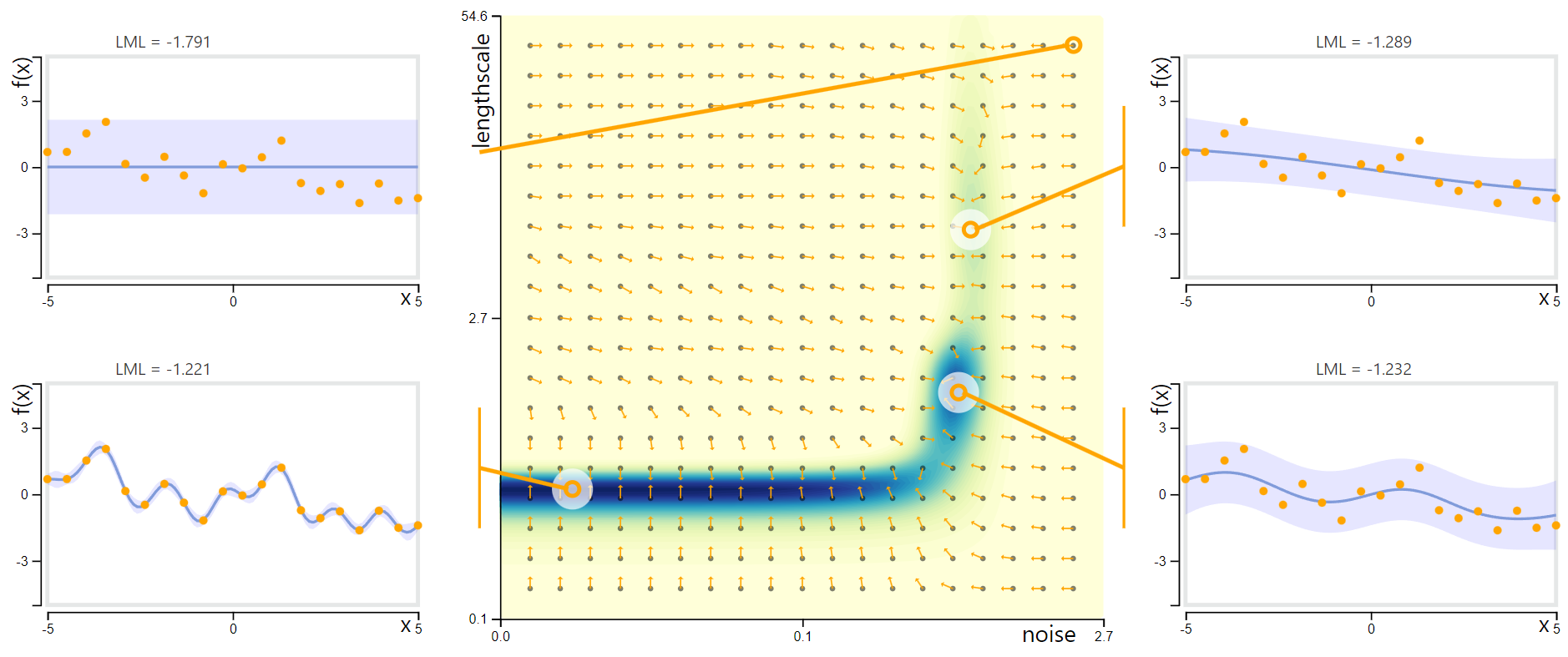Parameter Log Marginal Likelihood Landscape for GP Regression with RBF Kernel. Image source: Deisenroth et al., 2020. The outer scatterplots contain the same observed data (orange points) with GP models corresponding to different feasible parameterisations.

Centre: Objective landscape with contour of log marginal likelihood, for fixed signal variance $s$ with varying noise variances $\sigma^2$ and length scales $l$. Arrows show direction of gradient.
Upper left: This region of parameter space implies that the observed data is pure noise, with no discernible trend or signal. This parameterisation shows symptoms of underfitting and corresponds to the lowest log marginal likelihood of the four.
Upper right: This plot corresponds to large noise variance and large length scale, suggesting the data are sampled from a highly noisy and highly smooth base function, that is near linear at the scale plotted.
Lower left: This parameterisation implies that the data generating process is close to noiseless. The resulting model closely interpolates the observed data and corresponds to the global likelihood maximum, but may be deemed to be overfitting.
Lower right: A plausible middle-ground which aptly captures the general trend and interprets the data as noisy samples from a sinusoidal wave.

We have introduced the Gaussian process regression, which is applied in the context of supervised learning. In the supervised setting observations are labelled and our goal is to learn a posterior predictive distribution over the data, in order to infer the value of the output at a novel test input.

When working with large datasets in Gaussian Process models, consider using sparse approximations to improve computational efficiency without significant loss of accuracy.

Throughout the rest of this document, we instead consider an unsupervised setting, wherein we are concerned with data for which no specific output values or labels are provided. The primary objective is to infer latent structure within the data, with the aim to characterise the data generating process or to reduce data complexity for later statistical analyses.

Latent Variable Models for Dimensionality Reduction

Latent variable modelling is a powerful framework for interpreting high-dimensional data. By inferring latent structure, we can capture the intrinsic dimensionality of high-dimensional data and reduce the data to simplify statistical analyses.

Principal Components Analysis

We recall the quintessential technique in dimensionality reduction, principal components analysis (PCA), which seeks the particular linear combinations of features that capture dimensions of maximal variance within the data. These principal components equivalently seek to minimise the information loss or reconstruction error incurred during reduction, as well as maximising variance.

Definition: Principal components analysis. Suppose we have a centred and standardised matrix $\textbf{Y} \in \mathbb{R}^{N \times D}$. The principal components $\textbf{V} = {v_1, v_2, \ldots, v_P}$ are the sorted eigenvectors of the covariance matrix $\textbf{C} = 1/(N-1) \cdot \mathbf Y^T \mathbf Y \in \mathbb R^{D\times D}$, given in descending order of their corresponding \textit{explained variances} or eigenvalues $\Lambda = {\lambda_1, \lambda_2, \ldots, \lambda_P}$. We specify a number $p < D$ and construct a projection matrix $\textbf{W} = [ v_1 \ v_2 \ \cdots \ v_p ] \in \mathbb R^{D\times p}$ whose columns are the first $p$ eigenvectors from $\textbf{V}$. The $(N \times p)$-dimensional reduced data matrix $\mathbf T$ is obtained by the linear transformation $\textbf{T} = \textbf{YW}$.

Probabilistic PCA and Linear Latent Factor Models

A probabilistic interpretation of principal components analysis (PPCA) presented by Tipping and Bishop [1999], pursues maximum likelihood estimates of the coefficients in the linear combinations. This probabilistic approach yields a generative model capable of handling noisy or missing inputs.

Definition: Probabilistic PCA. Given the centred matrix of data $\textbf{Y} \in \mathbb{R}^{N \times D}$, we assume that each observation or row $\textbf{y}_n \in \mathbb R^{D}$, $(n=1,…,N),$ is generated from a latent variable $\textbf{x}_n \in \mathbb{R}^Q$ through a linear transformation and then corrupted by an additive Gaussian noise: \begin{equation} \textbf{y}_n = \textbf{W}\textbf{x}_n + \boldsymbol{\epsilon}_n, \quad \boldsymbol{\epsilon}_n \sim \mathcal{N}(\mathbf 0, \sigma^2\textbf{I}_D). \end{equation} Here $\textbf{W} \in \mathbb{R}^{D \times Q}$ is the matrix of the weights, and $\sigma^2$ is the variance of the isotropic Gaussian noise. The latent variables $\textbf{x}_n \sim \mathcal{N}(\mathbf 0, \mathbf I_Q)$ are independent draws from a standard normal. \end{definition}

The model parameters, $\textbf{W}$ and $\sigma^2$, are typically estimated via maximum likelihood estimation. Given these parameters, we have $\textbf{y}_n \mid \mathbf x_n, \mathbf W, \sigma^2 \sim \mathcal N(\textbf{W}\textbf{x}_n, \sigma^2\textbf{I}_D)$. By marginalising the latent variables $\mathbf x_n$ out of the joint distribution, we obtain a Gaussian distribution over $\textbf{y}_n$. In particular, we have $p(\mathbf y_n \mid \mathbf W, \sigma^2) = \int p(\mathbf y_n \mid \mathbf x_n, \mathbf W, \sigma^2) p(\mathbf x_n) d\mathbf x_n = \mathcal N(\mathbf 0, \textbf{WW}^T + \sigma^2\textbf{I}_D)$. Here the variance of the data is elegantly expressed as the sum of two components: $\textbf{WW}^T$ represents the portion of variance explained by the underlying latent structure of the data, and $\sigma^2\textbf{I}_D$ captures the residual variance which is independent of the latent variables and treated as isotropic Gaussian noise. However, probabilistic PCA and other linear latent factor models can be unsuitable in the case that nonlinear relationships are present in the data.

Gaussian Process Latent Variable Models (GPLVMs)

GPLVMs are a class of generative model that use principles of GP regression to learn low-dimensional latent manifolds that map to high-dimensional observed data spaces. Lawrence [2005] presents GPLVMs as a nonparametric nonlinear generalisation of PPCA. The goal here is different than in the standard GP regression. In that supervised setting, we placed a GP prior over the latent function in order to learn a posterior predictive distribution over unseen function outputs at novel test inputs by conditioning on the observed training data. However, in this unsupervised setting of latent variable modelling and dimensionality reduction, our focus is instead to learn low-dimensional representations that accurately capture the diversity of the observed data.

In the GPLVM, we specify a kernel function $\mathcal K(\mathbf x, \mathbf x’; \boldsymbol{\theta})$ and posit Gaussian process priors on each of the mappings between the input space and dimensions $d = 1,…,D$ of the observed data,

\[y_{n,d} = f_{d} (\mathbf x_n) + \varepsilon_n, \qquad f_{d} \mid \mathbf X, \boldsymbol{\theta} \sim \mathcal{GP}(\mathbf{0}, \ \mathcal K(\mathbf x, \mathbf x'; \ \boldsymbol{\theta})).\]

Unlike the supervised setting, the inputs here are unobserved. We include the latent vectors $\mathbf x_n$, i.e., the rows the latent matrix $\mathbf X = [\mathbf x_1, …, \mathbf x_N]^T \in \mathbb R^{N\times Q}$, in the set of model parameters to be learned. We assume that the covariance matrix $\mathbf S = \sigma^2 \mathbf I_N$ of the i.i.d. Gaussian noise terms $\varepsilon_n$ is isometric, i.e. proportional to the identity matrix and scaled by the noise variance parameter $\sigma^2$.

As in the standard GP regression, we marginalise out the function mappings and pursue point estimates for the optimal values of the model parameters $\mathbf X, \boldsymbol \theta,$ and $\sigma^2$ using MLE. Let $\mathbf K \in \mathbb R^{N\times N}$ denote the kernel matrix whose $(i,j)^{th}$ element is given by evaluating $\mathcal K(\mathbf x_i, \mathbf x_j; \ \boldsymbol{\theta})$. Under the assumption that the features $\mathbf y_d$ of the observed data $\mathbf Y$ are conditionally independent, given the latent variables $\mathbf X$, then the likelihood of the data under the GPLVM is formulated as the product over the columns $\mathbf y_d$ of $\mathbf Y$, $p(\mathbf Y \mid \mathbf X, \boldsymbol{\theta}, \sigma^2) = \prod_{d=1}^D p(\mathbf y_d \mid \mathbf X, \boldsymbol{\theta}, \sigma^2).$ The likelihood of the vector $\mathbf y_d$ is obtained by marginalising out the vector of function mappings $\mathbf f_d$:

\[p(\mathbf y_d \mid \mathbf X, \boldsymbol{\theta}, \sigma^2) = \int p(\mathbf y_d \mid \mathbf f_d, \mathbf X, \boldsymbol{\theta}, \sigma^2) \ p(\mathbf f_d \mid \mathbf X, \boldsymbol{\theta}) \ d \mathbf f_d = \mathcal N(\mathbf 0, \mathbf K + \mathbf S).\]

We see that the likelihood of the high-dimensional data $\mathbf Y$ is expressible a product of $D$-many conditionally independent Gaussian processes. That is, we are effectively considering a unique, conditionally independent regression on each feature or dimension. The log likelihood of the data $\mathbf Y$,

\[\begin{align} \log p(\mathbf Y \mid \mathbf X, \boldsymbol{\theta}, \sigma^2) &= \log \ \prod_{d=1}^D \ \mathcal N(\mathbf 0, \mathbf K + \mathbf S) \nonumber \\[.66em] &= \sum_{d=1}^D \log \left\{ \frac{1}{(2\pi)^{N/2} |\mathbf K + \mathbf S|^{1/2}} \exp{ \left( -\frac{1}{2} \mathbf y_d^T (\mathbf K+\mathbf S)^{-1} \mathbf y_d \right)} \right \} \nonumber \\[.66em] &= -\frac{D}{2} \log |\mathbf K+\mathbf S| - \frac{ND}{2} \log 2\pi - \frac{1}{2} \text{Tr}\left[ (\mathbf K+\mathbf S)^{-1} \mathbf Y\mathbf Y^T \right]. \end{align}\]

Given this formulation, we aim to determine optimal point estimates for $\mathbf X$, $\sigma^2$ and $\boldsymbol{\theta}$ which maximise the log-likelihood of the data.

We define the objective function $\mathcal L = - \log p(\mathbf Y \mid \mathbf X, \boldsymbol{\theta}, \sigma^2)$, which in this case is given as:

\[\begin{align} \mathcal L(\mathbf X, \boldsymbol{\theta}, \sigma^2 \mid \mathbf Y) = \frac{D}{2} \log |\mathbf K+\mathbf S| + \frac{ND}{2} \log 2\pi + \frac{1}{2} \text{Tr}\left[ (\mathbf K+\mathbf S)^{-1} \mathbf Y\mathbf Y^T \right]. \label{eqn:gplvm_obj_fnc} \end{align}\]

As in the standard GP regression, we use chain rule to compute the gradients of this negative log-likelihood $\mathcal L$ with respect to the latent variables $\mathbf X$ and the kernel parameters $\boldsymbol{\theta}$. From the definition of $\mathcal L$ above, we have the partial derivative of $\mathcal L$ w.r.t. $\mathbf K$:

\[\begin{align} \frac{\partial \mathcal L}{\partial \mathbf K} &= \frac{D}{2}(\mathbf K+\mathbf S)^{-1} - \frac{1}{2} (\mathbf{K}+\mathbf S)^{-1} \mathbf{Y}\mathbf{Y}^T (\mathbf{K}+\mathbf S)^{-1} \\[.5em] &= \frac{1}{2}[\mathbf K + \mathbf S]^{-1}\left( D [\mathbf K + \mathbf S] + \mathbf Y\mathbf Y^T)\right [\mathbf K + \mathbf S]^{-1}. \label{eqn:gplvm_dldk} \end{align}\]

By chain rule, we obtain our desired gradients,

\[\begin{align*} \frac{\partial \mathcal{L}}{\partial \mathbf{X}} = \frac{\partial \mathcal{L}}{\partial \mathbf{K}} \frac{\partial \mathbf{K}}{\partial \mathbf{X}}, \quad \text{and} \quad \frac{\partial \mathcal{L}}{\partial \boldsymbol{\theta}} = \frac{\partial \mathcal{L}}{\partial \mathbf{K}} \frac{\partial \mathbf{K}}{\partial \boldsymbol{\theta}}, \end{align*}\]

where the Jacobian matrices $\frac{\partial \mathbf K}{\partial X}$ and $\frac{\partial \mathbf K}{\partial \boldsymbol{\theta}}$ will depend on the specific kernel function specified. For example, the RBF kernel $\mathcal K_\text{RBF}$ is commonly used, which is parameterised by length scale $l$ and signal variance $s$.

We recall from the kernel table,

\[\mathcal K_\text{RBF}(\mathbf x, \mathbf x'; \boldsymbol l,s ) = s \exp \left( - \frac{1}{2l^2} ||\mathbf x - \mathbf x'|| \right).\]

The gradient of the RBF kernel w.r.t. the vector of parameters $\boldsymbol \theta = [l,s]$ is given by,

\[\nabla_{\boldsymbol \theta} \mathcal K_\text{RBF} = \left[\frac{\partial \mathcal K}{\partial l}, \frac{\partial \mathcal K}{\partial s}\right] = \left[ ||\mathbf x - \mathbf x'||^2 \left( \frac{s}{l^3}\right ) \exp \left(-\frac{1}{2l^2} ||\mathbf x - \mathbf x'||^2\right), \exp \left(-\frac{1}{2l^2} ||\mathbf x- \mathbf x'||^2\right) \right ].\]

As before, we optimise the noise variance parameter $\sigma^2$ by directly computing $\frac{\partial \mathcal L}{\partial \sigma^2}$:

\[\begin{align} \frac{\partial \mathcal L}{\partial \sigma^2} &= \frac{D}{2} \frac{\partial \log |\mathbf{K}+\mathbf{S}|}{\partial \sigma^2} + \frac{1}{2} \text{Tr}\left[\frac{\partial ([\mathbf{K}+\mathbf{S}]^{-1} \mathbf{Y}\mathbf{Y}^T)}{\partial \sigma^2}\right] \\[.5em] &= \frac{D}{2} \text{Tr}\left([\mathbf{K}+\mathbf{S}]^{-1}\right) - \frac{1}{2} \text{Tr}\left([\mathbf{K}+\mathbf{S}]^{-1} \mathbf{Y}\mathbf{Y}^T [\mathbf{K}+\mathbf{S}]^{-1}\right) \\[.5em] &= \frac{1}{2} \text{Tr} \left( D [\mathbf K + \mathbf S]^{-1} - [\mathbf K + \mathbf S]^{-1} \mathbf Y \mathbf Y^T [\mathbf K + \mathbf S]^{-1} \right) \\[.5em] &= \frac{1}{2} \text{Tr} \left([\mathbf K + \mathbf S]^{-1}\left( D [\mathbf K + \mathbf S] + \mathbf Y\mathbf Y^T)\right [\mathbf K + \mathbf S]^{-1} \right). \end{align}\]

Note, that the expression in previous line is simply the trace of the derived RHS of $\frac{\partial \mathcal L}{\partial \mathbf K}$ above, allowing for convenient and efficient reuse of computation. From here we can apply a gradient optimiser to obtain point estimates for the desired latent vectors $\mathbf X$, the kernel parameters $\boldsymbol \theta$ and noise variance $\sigma^2$. Note that in the case of a linear kernel and diagonal noise variance matrix, the GPLVM is equivalent to PPCA.

Python Comparison of PCA and GPLVM

In this section we will qualitatively compare PCA and GPLVMs using Python. For the GPLVMs we will use the GPy library, developed by the SheffieldML group: https://sheffieldml.github.io/GPy/. GPy is a lightweight high level API that allows quick and easy implementation of GP models akin to scikit-learn. For more in-depth problems, we may resort to other libraries such as GPyTorch or GPflow, (built on PyTorch and TensorFlow respectively), which allow for more granular control and customisation of the GP model formulation and training procedures.

These examples are generated using Python v3.8.16.

Beware: there is a known compatibility issue with GPy and numpy>=1.24:
See https://github.com/SheffieldML/GPy/issues/1004

  
import numpy as np
import pandas as pd
import seaborn as sns
import matplotlib.pyplot as plt
import GPy
np.random.seed(111) 

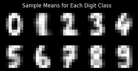
Here we consider the classic MNIST digits dataset.

  
from sklearn import datasets
mnist = datasets.load_digits()

# Compute sample means for each class
class_means = [
    np.mean(mnist.data[mnist.target == class_label], axis=0) 
    for class_label in range(10)
]

# Plotting those means
fig, axs = plt.subplots(2, 5, figsize=(5.5, 2.5), facecolor='black')
for class_label in range(10):
    col = class_label % 5
    row = class_label // 5
    axs[row, col].imshow(class_means[class_label].reshape((8, 8)), cmap='Greys_r')
    axs[row, col].axis('off')
fig.suptitle('Sample Means for Each Digit Class', size=12, color='white')
plt.show()

Training a GPLVM for MNIST Digits

In the following Python cell the object GPy.kern.RBF specifies a Radial Basis Function kernel. The method model.optimize(...) optimises the parameters of the model using gradient-based optimisation. In particular, we maximise the log marginal likelihood of the observed data, $p(\mathbf Y \mid \mathbf X, \theta, \sigma^2)$ with respect to the latent vectors $\mathbf X$, the kernel parameters $\theta$, and the noise variance $\sigma^2$, as discussed above.

  
from GPy.models import GPLVM
from GPy.kern import RBF

# Initialise kernel and model objects, and optimise for the MNIST dataset. 
model = GPLVM(mnist.data, input_dim=2, kernel = RBF(input_dim=2))
model.optimize(messages=True, max_iters=1e2)

We have succesfully applied the GPLVM to map the 64 dimensions of the MNIST pixels data down to simply 2 latent dimensions. We will now also construct a projection using principal components analysis for comparison.

  
from sklearn.decomposition import PCA
pca = PCA(n_components=2)
X_pca = pca.fit_transform(mnist.data)

# Axes to visualise the results of PCA vs GPLVM
fig, axs = plt.subplots(1, 2, figsize=(16,4.5))

# Plotting the PCA
sns.scatterplot(pd.DataFrame(X_pca, columns=['PC_1', 'PC_2']), 
                x='PC_1', y='PC_2', 
                hue=mnist.target.astype(str), 
                ax=axs[0],
                legend=None)
axs[0].set_title('PCA')

# Plotting the GPLVM
sns.scatterplot(pd.DataFrame(model.X.values, columns=['Dim_1','Dim_2']), 
                x='Dim_1', y='Dim_2', 
                hue=mnist.target.astype(str),
                ax=axs[1])
axs[1].set_title('GPLVM')
axs[1].legend(loc='upper left', bbox_to_anchor=(1, 1), title='Class')

plt.show()

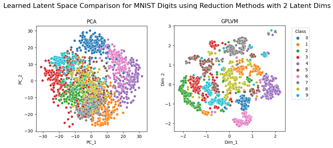Comparison of PCA and GPLVM on MNIST

Looking at these scatterplots, we can see quite clearly that the GPLVM model has managed to learn an ostensibly more useful latent space than the standard PCA. More specifically, with GPLVM we observe a greater degree of separability between the different classes as well as the formation of distinct clusters. By contrast PCA shows severe cluster overlap and it is challenging to predict where a new observation would likely be mapped to in the latent space.

Another method for evaluating the efficacy of our dimensionality reduction models is through the quality of reconstructions. In the context of our analysis, reconstruction involves first taking an observed sample from our dataset and learning a suitable point estimate for the corresponding latent vector. Then we pass the latent vector up through the mapping to the observed feature space. The degree of fidelity in these reconstructions serves as an insight into how well our models have captured the inherent structure of the data.

Once again we can see quite clearly that GPLVM significantly outperforms the PCA model. GPLVM has not only managed to preserve the core structure of the original observations, but also the finer details and clearly defined edges with accuracy.